Page 269 - Maxwell House

Chapter 5 249

th
> . As we have mentioned before, the positive δ indicates the zero delay in the N element
and maximum lag-delay in the zeroth element (see Figure 5.4.9 and 5.4.10). Evidently, it can
be arranged by sending the excitation wave in the direction z < 0 instead of z > 0, as before. If
so, the reverse in propagation may be taken into account by counting the elevation angle from
the axis z < 0 and thereby replacing → + in (5.89). It thus means that all plots in Figures
5.4.10 and 5.4.11 must be rotated 180°. Now the beam peaks lean to the left coming closer
toward the array z-axis in the direction of traveling wave propagation again.

5.4.8 Continuous Linear Array

The transition process to a linear array of a
continuous distribution of isotropic
radiators is quite straightforward. Let us
look back to expression (5.89) and assume
Sector of
Grating Lobes,
Discrete Array that the interelement separation reduces
while the number of elements + 1 in
array increases in such a way that the full
antenna length = is kept constant.

Putting as before that = − =

−(/ ) and = / we have for the

magnitude of normalized to the peak
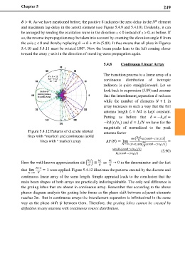
Figure 5.4.12 Patterns of discrete (dotted antenna factor
lines with *marker) and continuous (solid +1
lines with ° marker) array () = lim sin � (cos−/ )/2� =
→∞ (+1)sin � (cos−/ )/2�

sin ((cos−/ )/2)
(5.90)
(cos−/ )/2

Here the well-known approximation sin � � ≅ as → 0 in the denominator and the fact

+1
that lim = 1 were applied. Figure 5.4.12 illustrates the patterns created by the discrete and
→∞
continuous linear array of the same length. Simple appraisal leads to the conclusion that the
main beam shapes of both arrays are practically indistinguishable. The only real difference is
the grating lobes that are absent in continuous array. Remember that according to the above
phasor diagram analysis the grating lobe forms as the phase shift between adjacent elements
reaches 2. But in continuous arrays the interelement separation is infinitesimal in the same
way as the phase shift between them. Therefore, the grating lobes cannot be created by
definition in any antenna with continuous source distribution.