Page 270 - Maxwell House

250 ANTENNA BASICS

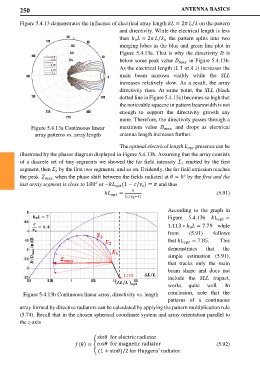
Figure 5.4.13 demonstrates the influence of electrical array length = 2 on the pattern
⁄
and directivity. While the electrical length is less
than = 2 the pattern splits into two
⁄
0
0
merging lobes as the blue and green line plot in
Figure 5.4.13a. That is why the directivity is
0.9
0.95 below some peak value in Figure 5.4.13b.
1
1.05
1.1 As the electrical length ( ↑ or ↓) increases the
1.15
1.2
main beam narrows visibly while the SLL
increases relatively slow. As a result, the array
directivity rises. At some point, the SLL (black
dotted line in Figure 5.4.13a) becomes so high that
the noticeable squeeze in pattern beamwidth is not
enough to support the directivity growth any
more. Therefore, the directivity passes through a
Figure 5.4.13a Continuous linear maximum value and drops as electrical
array patterns vs. array length antenna length increases further.

The optimal electrical length presence can be

illustrated by the phasor diagram displayed in Figure 5.4.13b. Assuming that the array consists
of a discrete set of tiny segments we showed the far field intensity emitted by the first
1
segment, then by the first two segments, and so on. Evidently, the far field emission reaches
2
the peak when the phase shift between the fields radiated at = 0° by the first and the
last array segment is close to 180° or − (1 − / ) = and thus

= (5.91)
⁄
( −1)
According to the graph in
Figure 5.4.13b =
1.113 ∗ = 7.79 while
0
from (5.91) follows
that = 7.85. This
demonstrates that the
simple estimation (5.91),
that tracks only the main
beam shape and does not
1.113
include the SLL impact,
works quite well. In
Figure 5.4.13b Continuous linear array, directivity vs. length conclusion, note that the
patterns of a continuous
array formed by directive radiators can be calculated by applying the pattern multiplication rule
(5.74). Recall that in the chosen spherical coordinate system and array orientation parallel to
the z-axis

sin for electric radiator
() = �cos for magnetic radiator (5.92)
(1 + sin)/2 for Huygens′ radiator