Page 332 - Maxwell House

312 Chapter 6

energy, let us look back at Figure 6.4.1 and 6.4.3d, and the equations (6.29) – (6.30) in Section
6.5.2 of this chapter. First of all, we need more information: namely the magnetic field structure.
There is no problem to continue our interpretation of wave mode propagation in WR as a
superposition of partial plane waves. It is a good approach, but it involves too many words and
drawings. So let us turn straight to Maxwell’s equation (6.3) and express the magnetic field
components through the known electrical vector (6.30). Since the only non-zero electrical
component is and / = −

(−)
= sin � � ⎫

0
⎪
= − sin (/) (−) (6.32)

0
0
⎬
/ (−) ⎪
= cos � �

0
0 ⎭
z
x
a y
b
x

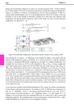
Figure 6.6.6 EM field configuration and surface electric current of TE -mode in WR
10
Note first that ≠ 0 and = 0. Therefore, (6.32) defines the family of TE-modes with the

uniform field distribution along y-coordinate. It is common practice to add the numerical
subscripts to distinguish WR modes assigning the subscript 0 to uniform distribution. For
example, the wave modes in (6.32) can be classified as TE 0 or H 0 . In more complicated
cases when partial waves reflect from all four WR walls the modes become TE (H ) or
TM (E ) depending of partial waves’ polarization. Evidently, each subscript is the half-

period number in transverse standing wave configuration. The dominant mode TE has the
10
largest critical wavelength = 2 meaning that the free propagation takes place in WR if and

only if the “door” opened by WR is “wider” than (“wave width”) or ≤ (see Section

6.4.3). The E- (green) and H- (medium purple) field force lines are demonstrated in Figure 6.6.6
as the whole 3D structure and its three cross-sections. Meanwhile, the surface electric current
(black) lines illustrate the net current continuity equation (1.64) from Chapter 1: the ends of
vector E proportional to the displacement current are the starting points for the conductivity
current and vice versa.
Let us look more carefully at the H-field polarization of TE -mode. We will use such data later
10
in this chapter analyzing ferrite devices. According to (6.32), H-field has two components

⁄
and in quadrature: () = −( ) sin (/) cos( − ) and () =

0
0

(( ) ) cos (/) sin( − ). Checking Figure 5.1.2 and Figure 5.1.3 in
⁄
⁄
0
0
Chapter 5 we can see that such two-component H-vector as a whole lays in the xz-plane and
elliptically polarized. The remarkable fact that this polarization switches from left- to right-
handed depending on the direction of wave propagation. Besides,