Page 178 - Servo Motors and Industrial Control Theory -

174 Appendix A

1
the maximum error occurs at frequency of with −3 db (amplitude ratio of
τ
0.7). And also show graphically that the phase lag can be approximated by a
straight line with slope of −45°/decade. The maximum error is at both ends of
the straight line with 5/6°.

θ i 1 θ o
τs + 1

42. The following block diagram shows a system with transfer function in the form
of a general second order lag. Similar to the previous example shown, the fre-
quency response when plotted in db against the frequency in logarithmic scaled
can be approximated by two straight lines. One at low frequency much smaller
than the natural frequency ω , with 0 db line. Another straight line at high fre-
n
quency much larger than ω with slope of 40 db per decade. The only correction
n
that must be added is at frequency near the natural frequency which depends on
the damping ratio. The correction can be made by knowing the damping ratio
1
(show that the maximum amplitude ratio is 2ξ and this occurs at frequency of
( ( ω n )· 1 ξ− 2 ) for damping ratio smaller than one. Also show that the phase lag
may also be approximated by a straight line with slope of 90° per decade. The
error depends on the damping ratio and it is minimum with damping ratio of
approximately between 0.5 and 1.

1
θ θ
i ξ  o
1   2 
ω  n  2 •s + 2  ω  •s + 1
n
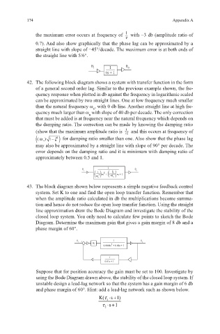
43. The block diagram shown below represents a simple negative feedback control
system. Set K to one and find the open loop transfer function. Remember that
when the amplitude ratio calculated in db the multiplications become summa-
tion and hence do not reduce the open loop transfer function. Using the straight
line approximation draw the Bode Diagram and investigate the stability of the
closed loop system. You only need to calculate few points to sketch the Bode
Diagram. Determine the maximum gain that gives a gain margin of 8 db and a
phase margin of 60°.

θ + 1 θ o
i K
2
- 0.0004s + 0.02s + 1
1
0.01s + 1
Suppose that for position accuracy the gain must be set to 100. Investigate by
using the Bode Diagram drawn above, the stability of the closed loop system. If
unstable design a lead-lag network so that the system has a gain margin of 6 db
and phase margin of 60°. Hint: add a lead-lag network such as shown below.
K(τ ⋅+
s 1)
1
τ ⋅+
s1
2