Page 9 - Handout Digital Electronics

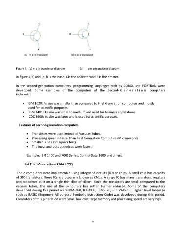
Figure 4: (a) n-p-n transistor diagram (b) p-n-p transistor diagram

In figure 4(a) and (b) B is the base, C is the collector and E is the emitter.

In the second-generation computers, programming languages such as COBOL and FORTRAN were
developed. Some examples of the computers of the Second- G e n e r a t i o n computers
included:

• IBM 1620: Its size was smaller than compared to First Generation computers and mostly
used for scientific purposes.
• IBM 1401: Its size was small to medium and used for business applications
• CDC 3600: Its size was large and is used for scientific purposes.

Features of second-generation computers

• Transistors were used instead of Vacuum Tubes.
• Processing speed is faster than First Generation Computers (Microsecond)
• Smaller in Size (51 square feet)
• The input and output devices were faster.

Example: IBM 1400 and 7000 Series, Control Data 3600 and others.

1.4 Third Generation (1964-1977)

These computers were implemented using integrated circuits (ICs) or chips. A small chip has capacity
of 300 transistors. These ICs are popularly known as Chips. A single IC has many transistors, registers
and capacitors built on a single thin slice of silicon. Since the transistors are small compared to the
vacuum tubes, the size of the computers has gotten further reduced. Some of the computers
developed during this period were IBM-360, ICL-1900, IBM-370, and VAX-750. Higher level language
such as BASIC (Beginners All-purpose Symbolic Instruction Code) was developed during this period.
Computers of this generation were small, low cost, large memory and processing speed are very high.

9