Page 490 - Microeconomics, Fourth Edition

c11monopolyandmonopsony.qxd 7/14/10 7:58 PM Page 464

464 CHAPTER 11 MONOPOLY AND MONOPSONY

MC (plant 1) MC (plant 2)
Profit- 1 2
maximizing
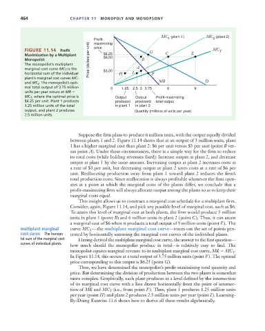
FIGURE 11.14 Profit price G MC T
Maximization by a Multiplant $6.25 C E
$6.00
Monopolist Price (dollars per unit) B
The monopolist’s multiplant
marginal cost curve MC T is the $3.00 A
horizontal sum of the individual H I F
plant’s marginal cost curves MC 1
and MC 2 . The monopolist’s opti- MR D
mal total output of 3.75 million 0 1.25 2.5 3 3.75 6 9
units per year occurs at MR
MC T , where the optimal price is Output Output Profit-maximizing
$6.25 per unit. Plant 1 produces produced produced total output
1.25 million units of the total in plant 1 in plant 2
output, and plant 2 produces Quantity (millions of units per year)
2.5 million units.

Suppose the firm plans to produce 6 million units, with the output equally divided
between plants 1 and 2. Figure 11.14 shows that at an output of 3 million units, plant
1 has a higher marginal cost than plant 2: $6 per unit versus $3 per unit (point B ver-
sus point A). Under these circumstances, there is a simple way for the firm to reduce
its total costs (while holding revenues fixed): Increase output at plant 2, and decrease
output at plant 1 by the same amount. Increasing output at plant 2 increases costs at
a rate of $3 per unit, but decreasing output at plant 2 saves costs at a rate of $6 per
unit. Reallocating production away from plant 1 toward plant 2 reduces the firm’s
total production costs. Since reallocation is always profitable whenever the firm oper-
ates at a point at which the marginal costs of the plants differ, we conclude that a
profit-maximizing firm will always allocate output among the plants so as to keep their
marginal costs equal.
This insight allows us to construct a marginal cost schedule for a multiplant firm.
Consider, again, Figure 11.14, and pick any possible level of marginal cost, such as $6.
To attain this level of marginal cost at both plants, the firm would produce 3 million
units in plant 1 (point B) and 6 million units in plant 2 (point C). Thus, it can attain
a marginal cost of $6 when it produces a total output of 9 million units (point E). The
multiplant marginal curve MC T —the multiplant marginal cost curve—traces out the set of points gen-
cost curve The horizon- erated by horizontally summing the marginal cost curves of the individual plants.
tal sum of the marginal cost Having derived the multiplant marginal cost curve, the answer to the first question—
curves of individual plants. how much should the monopolist produce in total—is relatively easy to find. The
monopolist equates marginal revenue to its multiplant marginal cost curve, MR MC T .
In Figure 11.14, this occurs at a total output of 3.75 million units (point F). The optimal
price corresponding to this output is $6.25 (point G).
Thus, we have determined the monopolist’s profit-maximizing total quantity and
price. But determining the division of production between the two plants is somewhat
more complex. Graphically, each plant produces at a level defined by the intersection
of its marginal cost curve with a line drawn horizontally from the point of intersec-
tion of MR and MC T (i.e., from point F). Thus, plant 1 produces 1.25 million units
per year (point H) and plant 2 produces 2.5 million units per year (point I ). Learning-
By-Doing Exercise 11.6 shows how to derive all these results algebraically.