Page 757 - Microeconomics, Fourth Edition

BMappAMathematicalAppendix.qxd 8/17/10 1:10 AM Page 731

A.1 FUNCTIONAL RELATIONSHIPS 731
if we want consumers to demand 4 million liters per year, For practice drawing supply and demand curves from
we should set the price at $8 per liter. To emphasize that P an equation, you might review Learning-By-Doing Exer-
is a function of Q, we might also write equation (A.3) as cises 2.1 and 2.2.
P(Q) 16 2Q.
When we draw a demand curve with P on the vertical LEARNING-BY-DOING EXERCISE A.1
axis and Q on the horizontal axis, the slope of the graph is
just the “rise over the run,” that is, the change in price (the Graphing Total Cost
vertical distance) divided by the change in quantity (the
horizontal distance) as we move along the curve. For exam- This example will help you see how to draw a graph and
ple, as we move from point S to point T, the change in price construct a table for a total cost function. Suppose that the
is P 2, and the change in quantity is Q 1. Thus, function representing the relationship between the total
the slope is P/ Q 2. Since the demand curve in costs of production (C) and the quantity produced (Q) is as
the example is a straight line, the slope is a constant every- follows:
where on the curve. The vertical intercept of the demand C(Q) Q 10Q 40Q (A.4)
3
2
curve occurs at point R, at a price of $16 per liter. This
means that no paint would be sold at that price or any Problem In a table, show the total cost of producing each
1
higher price. If the price of paint were zero, then people of the amounts of output: Q 0, Q 1, Q 2, Q 3,
would demand 8 million liters. This is the horizontal inter- Q 4, Q 5, Q 6, Q 7. Draw the total cost function
cept in the graph, at point Z. on a graph with total cost on the vertical axis and quantity
on the horizontal axis.
1 You may recall from a course in algebra that the equation of a Solution The first two columns of Table A.1 show the
straight line is y mx b , where y is plotted on the vertical axis total cost for each level of output. For example, to produce
and x is measured on the horizontal axis. With such a graph m is three units, we evaluate C(Q) when Q 3. We find that
2
3
the slope of the graph and b is the vertical intercept. In Figure A.1 C(3) (3) 10(3) 40(3) 57. (Do not worry about the
the “y” variable is P because it is plotted on the vertical axis and the other columns in the table. We will refer to them later.)
“x” variable (the one on the horizontal axis) is Q. Thus, instead The total cost curve is plotted in panel (a) in Figure A.2.
of having the equation y 2x 16 , with the example we have [Do not worry about panel (b). We will refer to it later.]
P 2Q 16 . The slope is 2 and the vertical intercept is 16.
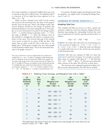
TABLE A.1 Relating Total, Average, and Marginal Cost with a Table*

(1) (2) (3) (4) (5)
Quantity Total “Arc” “Point” Average
Produced Cost Marginal Cost Marginal Cost Cost
(units) ($) ($/unit) ($/unit) ($/unit)
Q C C(Q) C(Q 1) dC/dQ C/Q

0 0 40
C(1) C(0) 31
1 31 23 31
C(2) C(1) 17
2 48 12 24
C(3) C(2) 9
3 57 7 19
C(4) C(3) 7
4 64 8 16
C(5) C(4) 11
5 75 15 15
C(6) C(5) 21
6 96 28 16
C(7) C(6) 37
7 133 47 19
*The table shows the values of total cost, marginal cost, and average cost curves when the cost
2
3
function is C(Q) Q 10Q 40Q.