Page 759 - Microeconomics, Fourth Edition

BMappAMathematicalAppendix.qxd 8/17/10 1:10 AM Page 733

A.2 WHAT IS A “MARGIN”? 733
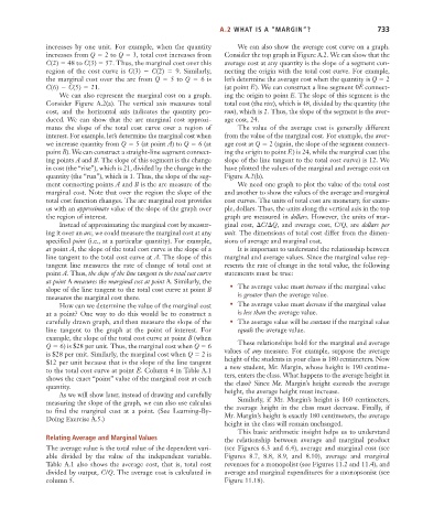
increases by one unit. For example, when the quantity We can also show the average cost curve on a graph.
increases from Q 2 to Q 3, total cost increases from Consider the top graph in Figure A.2. We can show that the
C(2) 48 to C(3) 57. Thus, the marginal cost over this average cost at any quantity is the slope of a segment con-
region of the cost curve is C(3) C(2) 9. Similarly, necting the origin with the total cost curve. For example,
the marginal cost over the arc from Q 5 to Q 6 is let’s determine the average cost when the quantity is Q 2
C(6) C(5) 21. (at point E). We can construct a line segment 0E connect-
We can also represent the marginal cost on a graph. ing the origin to point E. The slope of this segment is the
Consider Figure A.2(a). The vertical axis measures total total cost (the rise), which is 48, divided by the quantity (the
cost, and the horizontal axis indicates the quantity pro- run), which is 2. Thus, the slope of the segment is the aver-
duced. We can show that the arc marginal cost approxi- age cost, 24.
mates the slope of the total cost curve over a region of The value of the average cost is generally different
interest. For example, let’s determine the marginal cost when from the value of the marginal cost. For example, the aver-
we increase quantity from Q 5 (at point A) to Q 6 (at age cost at Q 2 (again, the slope of the segment connect-
point B). We can construct a straight-line segment connect- ing the origin to point E) is 24, while the marginal cost (the
ing points A and B. The slope of this segment is the change slope of the line tangent to the total cost curve) is 12. We
in cost (the “rise”), which is 21, divided by the change in the have plotted the values of the marginal and average cost on
quantity (the “run”), which is 1. Thus, the slope of the seg- Figure A.2(b).
ment connecting points A and B is the arc measure of the We need one graph to plot the value of the total cost
marginal cost. Note that over the region the slope of the and another to show the values of the average and marginal
total cost function changes. The arc marginal cost provides cost curves. The units of total cost are monetary, for exam-
us with an approximate value of the slope of the graph over ple, dollars. Thus, the units along the vertical axis in the top
the region of interest. graph are measured in dollars. However, the units of mar-
Instead of approximating the marginal cost by measur- ginal cost, C/ Q, and average cost, C/Q, are dollars per
ing it over an arc, we could measure the marginal cost at any unit. The dimensions of total cost differ from the dimen-
specified point (i.e., at a particular quantity). For example, sions of average and marginal cost.
at point A, the slope of the total cost curve is the slope of a It is important to understand the relationship between
line tangent to the total cost curve at A. The slope of this marginal and average values. Since the marginal value rep-
tangent line measures the rate of change of total cost at resents the rate of change in the total value, the following
point A. Thus, the slope of the line tangent to the total cost curve statements must be true:
at point A measures the marginal cost at point A. Similarly, the
• The average value must increase if the marginal value
slope of the line tangent to the total cost curve at point B
measures the marginal cost there. is greater than the average value.
How can we determine the value of the marginal cost • The average value must decrease if the marginal value
at a point? One way to do this would be to construct a is less than the average value.
carefully drawn graph, and then measure the slope of the • The average value will be constant if the marginal value
line tangent to the graph at the point of interest. For equals the average value.
example, the slope of the total cost curve at point B (when
Q 6) is $28 per unit. Thus, the marginal cost when Q 6 These relationships hold for the marginal and average
is $28 per unit. Similarly, the marginal cost when Q 2is values of any measure. For example, suppose the average
$12 per unit because that is the slope of the line tangent height of the students in your class is 180 centimeters. Now
to the total cost curve at point E. Column 4 in Table A.1 a new student, Mr. Margin, whose height is 190 centime-
shows the exact “point” value of the marginal cost at each ters, enters the class. What happens to the average height in
quantity. the class? Since Mr. Margin’s height exceeds the average
As we will show later, instead of drawing and carefully height, the average height must increase.
measuring the slope of the graph, we can also use calculus Similarly, if Mr. Margin’s height is 160 centimeters,
to find the marginal cost at a point. (See Learning-By- the average height in the class must decrease. Finally, if
Doing Exercise A.5.) Mr. Margin’s height is exactly 180 centimeters, the average
height in the class will remain unchanged.
This basic arithmetic insight helps us to understand
Relating Average and Marginal Values the relationship between average and marginal product
The average value is the total value of the dependent vari- (see Figures 6.3 and 6.4), average and marginal cost (see
able divided by the value of the independent variable. Figures 8.7, 8.8, 8.9, and 8.10), average and marginal
Table A.1 also shows the average cost, that is, total cost revenues for a monopolist (see Figures 11.2 and 11.4), and
divided by output, C/Q. The average cost is calculated in average and marginal expenditures for a monopsonist (see
column 5. Figure 11.18).