Page 760 - Microeconomics, Fourth Edition

BMappAMathematicalAppendix.qxd 8/17/10 1:10 AM Page 734

734 MATHEMATICAL APPENDIX
LEARNING-BY-DOING EXERCISE A.2 A.3 DERIVATIVES

Relating Average and Marginal Cost In Figure A.2, we showed that one way to find the marginal
cost is to plot the total cost curve and carefully measure the
This example will reinforce your understanding of the rela-
tionship between marginal and average values. Consider slope at each quantity. This is a tedious process, and it is not
the average and marginal cost curves in Figure A.2(b). always easy to draw a precise tangent line and measure its
slope accurately. Instead, we can use the powerful tech-
Problem Use the relationship between marginal and aver- niques of differential calculus to find the marginal cost or
age cost to explain why the average cost curve is rising, other marginal values we might want to know about.
falling, or constant at each of the following quantities: Let’s suppose that y is the dependent variable and x the
independent variable in a function:
(a) Q 2
y f (x)
(b) Q 5
(c) Q 6 Consider Figure A.3, which depicts the value of the
dependent variable on the vertical axis and the value of the
Solution independent variable on the horizontal axis.
(a) When Q 2, the marginal cost curve lies below the average As we have already discussed, if y measures the total
cost curve. Thus the average cost curve must be falling (have value, then the slope of the graph at any point measures the
a negative slope). marginal value. (For example, if y measures total cost and x
the quantity, then the slope of the cost function is the mar-
(b) When Q 5, the marginal cost curve is equal to the ginal cost at any quantity.) We can use a concept called a
average cost curve (they intersect). Thus the average cost derivative to help us find the slope of a function at any
curve must be neither increasing nor decreasing (have a point, such as point A in the figure.
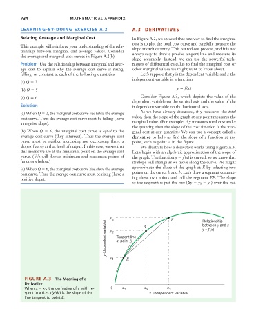
slope of zero) at that level of output. In this case, we see that We illustrate how a derivative works using Figure A.3.
this means we are at the minimum point on the average cost Let’s begin with an algebraic approximation of the slope of
curve. (We will discuss minimum and maximum points of the graph. The function y f (x) is curved, so we know that
functions below.) its slope will change as we move along the curve. We might
approximate the slope of the graph at E by selecting two
(c) When Q 6, the marginal cost curve lies above the average
cost curve. Thus the average cost curve must be rising (have a points on the curve, E and F. Let’s draw a segment connect-
positive slope). ing these two points and call the segment EF. The slope
of the segment is just the rise ( y y 3 y 1 ) over the run

y 3 B F Relationship
y (dependent variable) y 2 Tangent line y = f(x)
between y and x

at point E

y
1 E

FIGURE A.3 The Meaning of a
Derivative
When x x 1 , the derivative of y with re- 0 x 1 x 2 x 3
spect to x (i.e., dy/dx) is the slope of the x (independent variable)
line tangent to point E.