Page 122 - Computer Graphics Handout

3.10 CONCATENATION OF TRANSFORMATIONS

In this section, we create examples of affine transformations by multiplying together, or concatenating, sequences of the basic
transformations that we just introduced. Using this strategy is preferable to attempting to define an arbitrary transformation
directly. The approach fits well with our pipeline architectures for implementing
graphics systems.
Suppose that we carry out three successive transformations on a point p, creating a new point q. Because the matrix product is
associative, we can write the
sequence as

q = CBAp,
without parentheses. Note that here the matrices A, B, and C (and thus M) can be arbitrary 4×4 matrices, although in practice they
will most likely be affine. The order in which we carry out the transformations affects the efficiency of the calculation. In one view,
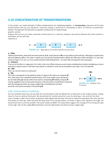
shown in Figure 3.43, we can carry out A, followed by B, followed by C—an order that corresponds to the grouping
q = (C(B(Ap))).
If we are to transform a single point, this order is the most efficient because each matrix multiplication involves multiplying a column
matrix by a square matrix. If we have many points to transform, then we can proceed in two steps. First, we calculate
M = CBA.
Then, we use this matrix on each point
q = Mp.
This order corresponds to the pipeline shown in Figure 3.44, where we compute M
first, then load it into a pipeline transformation unit. If we simply count operations,
we see that although we do a little more work in computing M initially, because M
may be applied to tens of thousands of points, this extra work is insignificant compared
with the savings we obtain by using a single matrix multiplication for each
point.We now derive examples of computing M.

3.10.1 Rotation About a Fixed Point
Our first example shows how we can alter the transformations that we defined with a fixed point at the origin (rotation, scaling,
shear) to have an arbitrary fixed point. We demonstrate for rotation about the z-axis; the technique is the same for the other
cases. Consider a cube with its center at pf and its sides aligned with the axes. We want to rotate the cube about the z-axis, but this
time about its center pf , which becomes the fixed point of the transformation, as shown in Figure 3.45. If pf were the origin, we
would know how to solve the problem: We would simply use Rz(θ). This observation suggests the strategy of first moving the cube
to the origin. We can then apply Rz(θ) and finally move the object back such that its center is again at pf .

122