Page 407 - Maxwell House

MORE COMPLICATED ELEMENTS OF FEED LINES 387

R c)
E
S
O
N
A
T
O
R

d)

a) b)

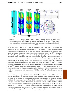
Figure 8.1.2 Coaxial in-line resonator: a) CST model, b) E-field distribution nearby and at
resonance frequency of 2.9 GHz, c) Insertion loss (dB) vs. frequency, d) Smith chart
showing the input impedance variations and three resonances over frequencies from 0
GHz to 10 GHz

34.50 mm) and 9.2 GHz (Λ = 22.50 mm), are clearly visible in Figure 8.1.2c with the plot
3
of the insertion loss. At each of these frequencies, the wave energy goes through the resonator
practically without reflections, i.e. the peak insertion loss is around 0dB. Note that the physical
length of resonator was chosen 29 mm meaning that its electrical length is 29√2.1 =42.02 mm.
Therefore, the capacitive gaps connected in series ( 11 > 0) lengthens the resonator at all these
frequencies in full agreement with (8.2). Smith chart in Figure 8.1.2d demonstrates that the
resonator input impedance switches around the resonance at 2.9 GHz (symbol ) from
inductive ( > , red top arrow) before the resonance to capacitive ( > , bottom red

arrow) after the resonance (the origin of chart). Thereby, it performs as parallel a ℒ circuit
connected in parallel as Figure 8.1.2c depicts. Meanwhile, the input impedance around 6 GHz
(symbol ) changes from capacitive to inductive (bottom and top green arrows) in the same
manner as the series ℒ circuit connected in series. Finally, the in-line resonator returns to the
parallel ℒ circuit connected in parallel at 9.2 GHz (symbol and dark magenta arrows
nearby).
The set of images in Figure 8.1.2b demonstrates the E-field distributions at 2.9 GHz and two
adjacent frequencies. The red color indicates the E-field peak while the little or no fields (-40
dB down) is marked in blue. At resonance frequency, E-field reaches its peaks over the gaps
and inside the resonator, as expected, and distributes almost as an ideal standing wave with the
node (but not exactly zero) in the resonator middle cross section. The top input and bottom
output fields are shown in light green are equal. The output E-field drops to -40 dB level at the
frequencies 2.4 GHz and 3.4 GHz meaning that the in-line resonator reflects the EM energy
back to the source. It is curious that mostly reactive E-field penetrates the resonator and even
reaches the bottom gap at both frequencies but cannot go through.