Page 865 - Mechatronics with Experiments

®
®
MATLAB , SIMULINK , STATEFLOW, AND AUTO-CODE GENERATION 851
Scope
0 +
1
–
Constant: input 10 x s 1
0 x s
Integrator
Initial velocity
Initial position Integrator 1
sin
x
Product Trigonometric
function
9.8/1.0
Constant 1: g/I term
®
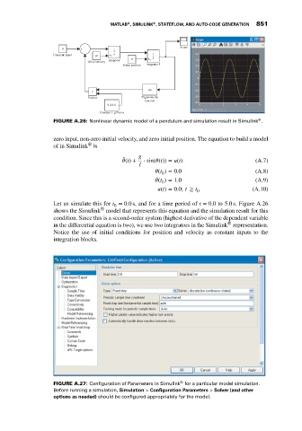
FIGURE A.26: Nonlinear dynamic model of a pendulum and simulation result in Simulink .

zero input, non-zero initial velocity, and zero initial position. The equation to build a model
®
of in Simulink is
g
̈
(t) + ⋅ sin( (t)) = u(t) (A.7)
l
(t ) = 0.0 (A.8)
0
̇
(t ) = 1.0 (A.9)
0
u(t) = 0.0; t ≥ t 0 (A.10)
Let us simulate this for t = 0.0 s, and for a time period of t = 0.0to5.0 s. Figure A.26
0
®
shows the Simulink model that represents this equation and the simulation result for this
condition. Since this is a second-order system (highest derivative of the dependent variable
®
in the differential equation is two), we use two integrators in the Simulink representation.
Notice the use of initial conditions for position and velocity as constant inputs to the
integration blocks.

®
FIGURE A.27: Configuration of Parameters in Simulink for a particular model simulation.
Before running a simulation, Simulation > Configuration Parameters > Solver (and other
options as needed) should be configured appropriately for the model.