Page 18 - Tlahuizcalli CB-30_Neat

B. Measurement of the muon’s speed To find the mean value of these time
measurements, along with its corresponding
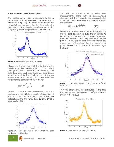
The distribution of time measurements for a standard deviation, a gaussian curve was adjusted
separation of 50cm between the detectors, is to this distribution, meaning the curve had to follow
presented in fig. (19). The scale of the bins in the the equation
horizontal axis was converted into time units with − ( )
1 − 2
the help of the calibration previously made (fig. ( ) = 2 , (15)
(10)): every channel represents (1/83.6183) .
Where is the mean value of the distribution, is
the standard deviation, and is the amplitude. As
in the previous experiment, the curve_fit function
from the Python library SciPy was used for this
purpose. In fig. (21) the best curve fit is shown. The
mean value of the distribution was found to be
= 15.685 , with standard deviation =
1
1
0.785 .

Figure 19. Time distribution for = 50 .
1
Based on the irregularity of the distribution, the
possibility of the presence of a non-constant
background was considered. To identify it, only
data from short and large times was considered,
since the peak in the middle of the distribution
wouldn’t allow to isolate the background. The
model for the background curve fit was

− Figure 21. Gaussian curve fit for the = 50
1
( ) = , (14) distribution.

On the other hand, the distribution of the time
Where , and were parameters. Once the measurements for a separation of = 100 is
background was obtained as a function of time, it shown in the fig. (22) 2
was subtracted from the data, and the resulting
distribution within the range from 12 to 19 is
shown in fig. (20).

Figure 20. Time distribution for = 50 after Figure 22. Time distribution for = 100 .
2
1
background subtraction.
17
Tlahuizcalli ISSN: 2448-7260 Año 10 Núm. 30 septiembre-diciembre 2024