Page 14 - Tlahuizcalli CB-30_Neat

After registering enough measurements to get a offset will cancel out of the equation when taking
time distribution, the distance between the the difference, as long as the experimental setup
scintillators was changed, and the time was remains the same for both measurements. This
measured again. means that the time resolution of the equipment
won’t be crucial, since the signals can be delayed
as long as necessary, and it won’t affect the
calculations.

The circuit layout employed for this experiment is
shown in fig. (9). The output signals from the PMTs
were introduced to a Linear Fan-in/Fan-out just as
an intermediate module. From here, both signals
were sent to discriminators where they were
converted into logic pulses. After that, the signals
were introduced into Gate & Delay generators,
where only the signal corresponding to the lower
detector was delayed by 8 . The non-delayed
signal was used as the START of the TAC, and the
delayed one was used as the STOP. The output
signal of the TAC was then sent to the MCA to
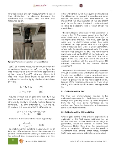
Figure 8. Vertical configuration of the scintillators. register its amplitude with the help of the same USX
software employed in the muon’s lifetime
Let be the time measured for a muon when the experiment.
1
separation of the detectors is ; and let be the
2
1
The pulses from both PMTs were being monitored
time measured for a muon when the separation is through an oscilloscope with higher time resolution
. We can write and as the sum of the actual than the one used in the previous experiment, since
1
2
2
time that takes each muon to go from one in this case, the time difference between the
scintillator to the other, , , plus the added delay observed pulses was in the nanoseconds scale,
2
1
= 8 instead of the microseconds scale as it was when
dealing with the decay of the muon (see Appendix
= + , (9) B).
1
1
= + . (10) B1. Calibration of the PMT
2
2
Assume without loss of generality that < ; This time two photomultipliers needed to be
1
2
then, because it takes for the muon to travel a calibrated separately. As in the first experiment, the
1
voltage was gradually turned up while the pulses
distance , and to travel , the time it requires from the PMT were being monitored on the
2
2
1
to travel − is the difference − . Using eq. oscilloscope. The optimal operating voltages were
1
1
2
2
(9) and eq. (10) we can write this difference as: set to 1.28kV for both PMTs.
= − = − − ( − ) B2. Calibration of the TAC and MCA
2
1
1
2
= − . (11)
2
1
Once again, just like in the previous experiment, a
Therefore, the velocity of the muon is given by calibration of the TAC signals registered by the
MCA was required, so that the bins of the histogram
− generated, could be related to actual time
= 2 1 . (12)
− 1 differences. Notice that, since the experimental
2
Eq. (12) shows that by taking measurements for at setup is completely different from the previous
least two different separations of the detectors, it is experiment and, among other things, different
possible to calculate the velocity of the muons with PMT’s were used, a new calibration was needed.
the delayed time measurements, since any time
13
Tlahuizcalli ISSN: 2448-7260 Año 10 Núm. 30 septiembre-diciembre 2024