Page 17 - Tlahuizcalli CB-30_Neat

Where the parameters to be adjusted are and
0
(which represents the background), while is
0

now fixed and set to the value = 2.2 , which

is the expected value. The resulting curve is shown
in fig. (14). A value for the background of =
0
406.512 ± 5.459 was obtained.

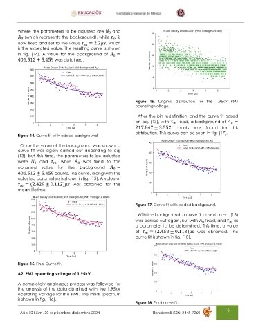
Figure 16. Original distribution for the 1.95kV PMT
operating voltage.

After the bin redefinition, and the curve fit based
on eq. (13), with fixed, a background of =

0
217.847 ± 3.552 counts was found for this
distribution. This curve can be seen in fig. (17).
Figure 14. Curve fit with added background.
Once the value of the background was known, a
curve fit was again carried out according to eq.
(13), but this time, the parameters to be adjusted
were and , while was fixed to the
0

0
obtained value for the background =
0
406.512 ± 5.459 counts. The curve, along with the
adjusted parameters is shown in fig. (15). A value of
= (2.429 ± 0.112) was obtained for the

mean lifetime.

Figure 17. Curve fit with added background.

With the background, a curve fit based on eq. (13)
was carried out again, but with fixed, and as

0
a parameter to be determined. This time, a value
of = (2.458 ± 0.113) was obtained. The

curve fit is shown in fig. (18).

Figure 15. Final Curve fit.

A2. PMT operating voltage of 1.95kV

A completely analogous process was followed for
the analysis of the data obtained with the 1.95kV
operating voltage for the PMT. The initial spectrum
is shown in fig. (16).
Figure 18. Final curve fit.

16
Año 10 Núm. 30 septiembre-diciembre 2024 Tlahuizcalli ISSN: 2448-7260