Page 637 - Microeconomics, Fourth Edition

c15riskandinformation.qxd 8/16/10 11:10 AM Page 611

15.2 EVALUATING RISKY OUTCOMES 611

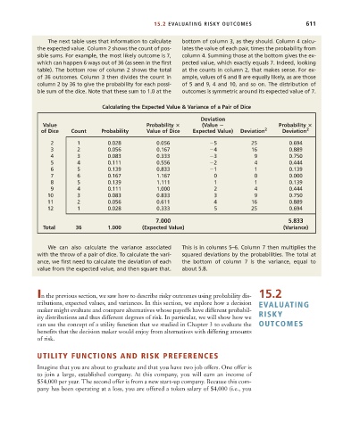
The next table uses that information to calculate bottom of column 3, as they should. Column 4 calcu-
the expected value. Column 2 shows the count of pos- lates the value of each pair, times the probability from
sible sums. For example, the most likely outcome is 7, column 4. Summing those at the bottom gives the ex-
which can happen 6 ways out of 36 (as seen in the first pected value, which exactly equals 7. Indeed, looking
table). The bottom row of column 2 shows the total at the counts in column 2, that makes sense. For ex-
of 36 outcomes. Column 3 then divides the count in ample, values of 6 and 8 are equally likely, as are those
column 2 by 36 to give the probability for each possi- of 5 and 9, 4 and 10, and so on. The distribution of
ble sum of the dice. Note that these sum to 1.0 at the outcomes is symmetric around its expected value of 7.

Calculating the Expected Value & Variance of a Pair of Dice

Deviation
Value Probability (Value Probability
of Dice Count Probability Value of Dice Expected Value) Deviation 2 Deviation 2

2 1 0.028 0.056 5 25 0.694
3 2 0.056 0.167 4 16 0.889
4 3 0.083 0.333 3 9 0.750
5 4 0.111 0.556 2 4 0.444
6 5 0.139 0.833 1 1 0.139
7 6 0.167 1.167 0 0 0.000
8 5 0.139 1.111 1 1 0.139
9 4 0.111 1.000 2 4 0.444
10 3 0.083 0.833 3 9 0.750
11 2 0.056 0.611 4 16 0.889
12 1 0.028 0.333 5 25 0.694

7.000 5.833
Total 36 1.000 (Expected Value) (Variance)

We can also calculate the variance associated This is in columns 5–6. Column 7 then multiplies the
with the throw of a pair of dice. To calculate the vari- squared deviations by the probabilities. The total at
ance, we first need to calculate the deviation of each the bottom of column 7 is the variance, equal to
value from the expected value, and then square that. about 5.8.

In the previous section, we saw how to describe risky outcomes using probability dis- 15.2
tributions, expected values, and variances. In this section, we explore how a decision EVALUATING
maker might evaluate and compare alternatives whose payoffs have different probabil-
ity distributions and thus different degrees of risk. In particular, we will show how we RISKY
can use the concept of a utility function that we studied in Chapter 3 to evaluate the OUTCOMES
benefits that the decision maker would enjoy from alternatives with differing amounts
of risk.

UTILITY FUNCTIONS AND RISK PREFERENCES

Imagine that you are about to graduate and that you have two job offers. One offer is
to join a large, established company. At this company, you will earn an income of
$54,000 per year. The second offer is from a new start-up company. Because this com-
pany has been operating at a loss, you are offered a token salary of $4,000 (i.e., you