Page 20 - FINAL CFA II SLIDES JUNE 2019 DAY 4

LOS 12.e: READING 11: CURRENCY EXCHANGE RATES: UNDERSTANDING EQUILIBRIUM VALUE
Forecast potential GDP based on growth accounting relations.

MODULE 12.1: GROWTH FACTORS AND PRODUCTION FUNCTION
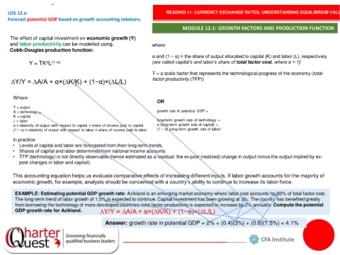
The effect of capital investment on economic growth (Y)
and labor productivity can be modelled using, where:
Cobb-Douglas production function:
α and (1 − α) = the share of output allocated to capital (K) and labor (L), respectively
α (1–α)
Y = TK L (are called capital’s and labor’s share of total factor cost, where α < 1]
T = a scale factor that represents the technological progress of the economy (total
∆Y/Y = ∆A/A + α×(∆K/K) + (1−α)×(∆L/L) factor productivity (TFP))

Where:
OR
Y = output
A = technology growth rate in potential GDP =
K = capital
L = labor long-term growth rate of technology +
α = elasticity of output with respect to capital = share of income paid to capital α (long-term growth rate of capital) +
(1 − α) = elasticity of output with respect to labor = share of income paid to labor (1 − α) (long-term growth rate of labor)
In practice:
• Levels of capital and labor are forecasted from their long-term trends,
• Shares of capital and labor determined from national income accounts.
• TFP (technology) is not directly observable (hence estimated as a residual: the ex-post (realized) change in output minus the output implied by ex-
post changes in labor and capital).

This accounting equation helps us evaluate comparative effects of increasing different inputs. If labor growth accounts for the majority of
economic growth, for example, analysts should be concerned with a country’s ability to continue to increase its labor force.

EXAMPLE: Estimating potential GDP growth rate: Azikland is an emerging market economy where labor cost accounts for 60% of total factor cost.
The long-term trend of labor growth of 1.5% is expected to continue. Capital investment has been growing at 3%. The country has benefited greatly
from borrowing the technology of more developed countries; total factor productivity is expected to increase by 2% annually. Compute the potential
GDP growth rate for Azikland. ∆Y/Y = ∆A/A + α×(∆K/K) + (1−α)×(∆L/L)

Answer: growth rate in potential GDP = 2% + (0.4)(3%) + (0.6)(1.5%) = 4.1%