Page 26 - PowerPoint Presentation

LOS 34.k: Describe modern term structure READING 34: THE TERM STRUCTURE AND
models and how they are used. INTEREST RATE DYNAMICS
MODULE 34.6: INTEREST RATE MODELS

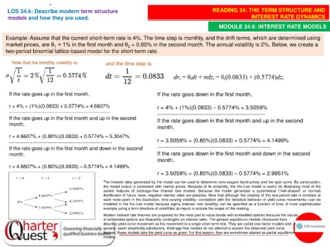
Example: Assume that the current short-term rate is 4%. The time step is monthly, and the drift terms, which are determined using
market prices, are θ = 1% in the first month and θ = 0.80% in the second month. The annual volatility is 2%. Below, we create a
1
2
two-period binomial lattice-based model for the short-term rate.

If the rate goes up in the first month, If the rate goes down in the first month,

r = 4% + (1%)(0.0833) + 0.5774% = 4.6607% r = 4% + (1%)(0.0833) – 0.5774% = 3.5059%
------------------------------------------------------------- -----------------------------------------------------------
If the rate goes up in the first month and up in the second If the rate goes down in the first month and up in the second
month,
month,
r = 4.6607% + (0.80%)(0.0833) + 0.5774% = 5.3047%
-------------------------------------------------------------- r = 3.5059% + (0.80%)(0.0833) + 0.5774% = 4.1499%
If the rate goes up in the first month and down in the second --------------------------------------------------------------
month, If the rate goes down in the first month and down in the second
month,
r = 4.6607% + (0.80%)(0.0833) – 0.5774% = 4.1499%
r = 3.5059% + (0.80%)(0.0833) – 0.5774% = 2.9951%

The interest rates generated by the model can be used to determine zero-coupon bond prices and the spot curve. By construction,
the model output is consistent with market prices. Because of its simplicity, the Ho–Lee model is useful for illustrating most of the
salient features of arbitrage-free interest rate models. Because the model generates a symmetrical (“bell-shaped” or normal)
distribution of future rates, negative interest rates are possible. Note that although the volatility of the one-period rate is constant at
each node point in the illustration, time-varying volatility—consistent with the historical behavior of yield curve movements—can be
modeled in the Ho–Lee model because sigma (interest rate volatility) can be specified as a function of time. A more sophisticated
example using a term structure of volatilities as inputs is outside the scope of this reading.
Modern interest rate theories are proposed for the most part to value bonds with embedded options because the values
of embedded options are frequently contingent on interest rates. The general equilibrium models introduced here
describe yield curve movement as the movement in a single short-term rate. They are called one-factor models and, in
general, seem empirically satisfactory. Arbitrage-free models do not attempt to explain the observed yield curve.
Instead, these models take the yield curve as given. For this reason, they are sometimes labeled as partial equilibrium
models.