Page 349 - Six Sigma Advanced Tools for Black Belts and Master Black Belts

OTE/SPH
OTE/SPH
Char Count= 0
3:7
August 31, 2006
JWBK119-21
334 Establishing Cumulative Conformance Count Charts
UCL
Warning zone
UDL
4 consecutive
points on one side 1 point within the
of the center line CL warning zone
(CL)

LDL
Warning zone
LCL

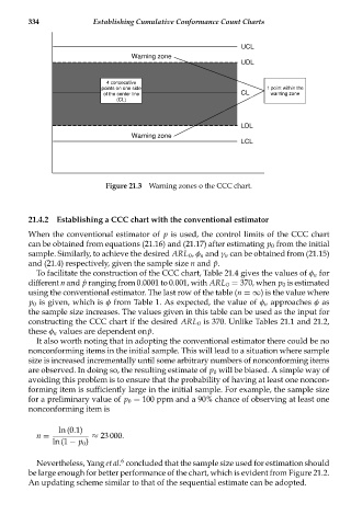
Figure 21.3 Warning zones o the CCC chart.

21.4.2 Establishing a CCC chart with the conventional estimator

When the conventional estimator of p is used, the control limits of the CCC chart
can be obtained from equations (21.16) and (21.17) after estimating p 0 from the initial
sample. Similarly, to achieve the desired ARL 0 , φ n and γ n can be obtained from (21.15)
and (21.4) respectively, given the sample size n and ˆp.
To facilitate the construction of the CCC chart, Table 21.4 gives the values of φ n for
different n and ˆp ranging from 0.0001 to 0.001, with ARL 0 = 370, when p 0 is estimated
using the conventional estimator. The last row of the table (n =∞) is the value where
p 0 is given, which is φ from Table 1. As expected, the value of φ n approaches φ as
the sample size increases. The values given in this table can be used as the input for
constructing the CCC chart if the desired ARL 0 is 370. Unlike Tables 21.1 and 21.2,
these φ n values are dependent on ˆp.
It also worth noting that in adopting the conventional estimator there could be no
nonconforming items in the initial sample. This will lead to a situation where sample
size is increased incrementally until some arbitrary numbers of nonconforming items
are observed. In doing so, the resulting estimate of p 0 will be biased. A simple way of
avoiding this problem is to ensure that the probability of having at least one noncon-
forming item is sufficiently large in the initial sample. For example, the sample size
for a preliminary value of p 0 = 100 ppm and a 90% chance of observing at least one
nonconforming item is

ln (0.1)
n = ≈ 23 000.
ln (1 − p 0 )

6
Nevertheless, Yang et al. concluded that the sample size used for estimation should
be large enough for better performance of the chart, which is evident from Figure 21.2.
An updating scheme similar to that of the sequential estimate can be adopted.