Page 351 - Six Sigma Advanced Tools for Black Belts and Master Black Belts

OTE/SPH
OTE/SPH
Char Count= 0
August 31, 2006
3:7
JWBK119-21
336 Establishing Cumulative Conformance Count Charts
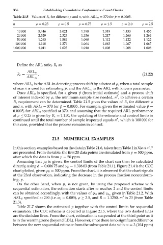
Table 21.5 Values of R c for different ρ and n, with ARL 0 = 370 for ˆp = 0.0005.
n ρ = 0.25 ρ = 0.5 ρ = 0.75 ρ = 1.5 ρ = 2.0 ρ = 2.5
10 000 5.446 3.021 1.198 1.319 1.433 1.455
20 000 2.529 2.323 1.156 1.217 1.260 1.264
50 000 1.293 1.584 1.098 1.112 1.122 1.122
100 000 1.118 1.279 1.064 1.063 1.067 1.067
1 000 000 1.011 1.025 1.010 1.008 1.008 1.008

Define the ARL ratio, R c as

ARL n
R c = , (21.22)
ARL ∞
where ARL n is the ARL in detecting process shift by a factor of ρ, when a total sample
of size n is used for estimating p, and the ARL ∞ is the ARL with known parameter.
Once ARL 0 is specified, for a given ˆp (from initial estimate) and a process shift
of interest indexed by ρ, the minimum sample size needed, n * , to achieve a certain
R c requirement can be determined. Table 21.5 gives the values of R c for different ρ
and n, with ARL 0 = 370 for ˆp = 0.0005. For example, given the estimated value ˆp =
0.0005, for ARL 0 specified at 370, and assuming that the required ARL performance
at ρ ≤ 0.25 is given by R c = 1.150, the updating of the estimate and control limits is
continued until the total number of sample inspected equals n * , which is 100 000 for
this case, provided that the process remains in control.

21.5 NUMERICAL EXAMPLES

In this section, examples based on the data in Table 21.6, taken from Table I in Xie et al., 5
are presented. From the table, the first 20 data points are simulated from p = 500 ppm,
after which the data is from p = 50 ppm.
Assuming that p 0 is given, the control limits of the chart can then be calculated
directly, using φ = 0.006 75 and γ φ = 1.306 03 (from Table 21.1). Figure 21.4 is the CCC
chart plotted, given p 0 = 500 ppm. From the chart, it is observed that the chart signals
at the 23rd observation, indicating the decrease in the process fraction nonconform-
ing, p.
On the other hand, when p 0 is not given, by using the proposed scheme with
sequential estimation, the estimation starts after m reaches 2 and the control limits
given in Table 21.2. With
can be obtained accordingly, with the values of φ m and γ φ m
ARL 0 specified at 200 (i.e. α 0 = 0.005), ρ ≥ 2.5, and R = 1.1250, m * is 23 (from Table
21.3).
Table 21.7 shows the estimated p together with the control limits for sequential
estimation. The CCC scheme is depicted in Figure 21.5, where the two dashed lines
are the decision lines. From the chart, estimation is suspended at the third point as it
is in the warning zone (beyond LDL). However, since there is no significant difference
between the new sequential estimate from the subsequent data with m = 3 (104 ppm)