Page 413 - Maxwell House

MORE COMPLICATED ELEMENTS OF FEED LINES 393

3. From the above discussion follows that the S-matrix of an ideal directional coupler can be
represented in the matrix form = like (8.4) or more detailly as

1 0 21 31 0 1
0 0
2
� � = � 21 21 � � 2 � (8.5)
3 31 0 0 21 3
4 0 31 21 0 4
4. The realized coupling factor (C) is equal (in relative units) to = 1/ 31 = ( ++ − )/
±

±
2
2
( ++ + ) = (( ++ / ) − 1) (( ++ / ) + 1).
⁄

5. Typically, the coupling factor and characteristic impedance are the given values. Then

++ 2
from the later expression we should find the even-mode impedance ( / ) = (1 +

2
±
±
)/(1 − ) and thus ( / ) = (1 − )/(1 + ). Therefore, ++ / = (1 + )/

(1 − ). This ratio is plotted in Figure 8.2.3b. It is clear that there are some technical
problems to develop coupling factor of 3 - 5 dB or less. For example, 3dB coupler
±
requires ++ / = 5.8284. Looking back at Figure 8.2.3a, we could come to conclusion

that we theoretically might design such coupler using only extremely narrow gap (s/d <
0.01) between traces but the fabrication of such couplers is problematic.
6. There are several ways to increase coupling between traces turning to striplines with a

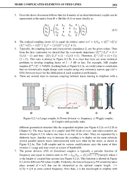
Figure 8.2.4 a) Lange coupler, b) Power division vs. frequency, c) Wiggly coupler,
d) Coupler with periodic stubs

different geometrical structure like the suspended stripline (see Figure 6.2.2c or 6.2.2h in
Chapter 6). The trace layout of a coupler and EM fields of even- and odd-excitation are
shown in Figure 8.2.3c where one trace is on top of the other. They are separated by a
dielectric layer. Another way to increase the coupling is to deploy on the same substrate
several parallel narrow traces interconnected with each other by the wires, as shown in
Figure 8.2.4a. This 3-dB coupler and its various modifications carry the name of their
inventor J. Lange and may cover an octave of bandwidth.
7. The power division (PD) of directional couplers is typically a periodic function of

2
frequency and equal in relative units to = / 31 = �/√1 − � tan() where
21
is the length of coupled line section (see Figure 8.2.2). This function is plotted in Figure
8.2.4b for different PD values in [dB]. Evidently, the lowest frequency PD sensitivity takes
place around = /2 that can be interpreted as the optimal coupler length =
2 = /4 at some central frequency. Here than, is the wavelength in stripline with
⁄